It’s not such a long time ago that oscilloscopes were once the reserve of scientists, with their use mainly focused on measuring complex signals in laboratories. As we all know, though, the cost of sophisticated technology reduces over time to such an extent that things that were once very expensive are now within our grasp.
Oscilloscopes are now quite affordable as a general measuring device, and can be particularly useful for automotive electrical and electronic system diagnostics; in fact, they’re now almost down to the price of a really good multimeter.
But, just because they’re within the practical reach of the automotive technician, does that mean it’s worth digging deep to invest in one? Even if you did, would you be able get any real benefit out if it? This feature hopes to enlighten you about what a scope can do for you – and your business – to help you make an informed decision about whether it’s worth taking the plunge.
Oscilloscopes: the basics
So, you’ve probably heard the term ‘oscilloscope’, but do you know what we’re actually talking about? Well, fundamentally, the ‘scope, as it’s commonly known, is a voltmeter; however, it gives a different view compared to the voltage displayed on a digital or analogue voltmeter, as this is normally given as a single reading or value – either via a needle on a scale, or as a discrete value.
In contrast, the reading given by a scope is a curve, drawn on a display screen – but how does this help you? Well, if a signal is displayed in this way – as a curve over time – it means that very fast moving changes can be displayed and visualised. For example, consider a signal in the form of a single voltage pulse, like a spike!
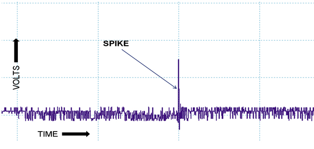
A spike couldn’t be seen on a meter, but on a scope display it’s very clear
If you looked at this signal on a digital multimeter it probably wouldn’t even register, as the meter sampling time is too slow. Looking via an analogue meter you may, if you’re lucky, see the needle twitch; however, look at the signal on a properly set up scope and you will see all the detail of the signal: the profile of the signal shape, the rising and falling edges, the peak value, plus the duration of the pulse.
In summary then, you have access to much more detail that you would likely miss by just using a meter.
Of course, there are some signals where you don’t need all that detail, especially where the signals are changing slowly over time; a temperature signal or manifold pressure sensor signal are good examples of this and it is fine to just view these with a meter.
However, signals which are dynamic in nature – those related to crank position, or fast changing sensor values in particular – make much more sense when viewed on a scope. To give a specific example: think of a crank position sensor signal.
View this signal on a meter and you’ll just see a constant or slightly wavering voltage; however, if you measure this with a scope, you’ll see all the details of the edges relating to crank position and the missing tooth relating to a TDC reference mark.
A signal such as this needs a scope measurement to really be able to check the signal quality during operation. If you were using a meter, you’d be hard-pressed to diagnose any run-time faults.
Scopes – analogue, then digital
As mentioned earlier, scopes were originally used in labs for analysing complex signal wave forms. In their earliest form, they were analogue devices, similar in many ways to the old-fashioned analogue television with a ‘tube’ inside. Basic operation was that an electron beam was fired at a cathode screen, drawing a straight line across the screen at regular intervals – according to the scope time base set-up.
This line was projected across the screen and displayed until it was redrawn – a very cyclic process, with the screen acting as a kind of short term memory. The beam would be deflected by the applied signal to be measured. Imagine a pulse: this would deflect the beam, and the line drawn on the screen would show the pulse pattern over time as the line is drawn across the screen.
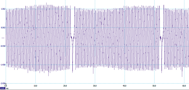
An example complex waveform (crank position sensor) – ideal for scope analysis
The disadvantage of this type of device is that it is difficult to store or capture a waveform; the only possible method is to literally photograph the screen image – not ideal!
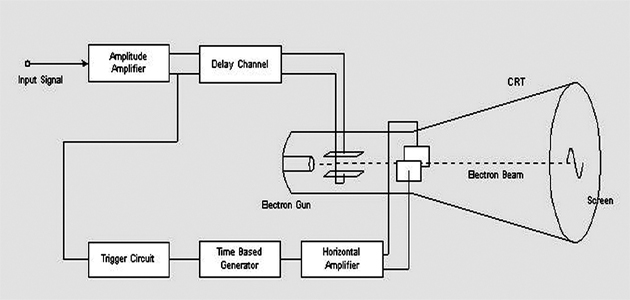
The basic principles of an analogue scope
The digital age overcame this by sampling a waveform and storing it digitally. With this technology, measurements can be stored in memory and further analysis can be carried out by a signal processor, either during or after the measurement. Wave forms can be archived as files on a hard disc drive, and then these digitally captured traces can be analysed in greater detail after the measurement.
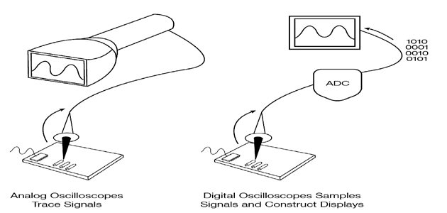
A comparison of analogue and digital scopes (source: Tektronix)
Digital scopes are now standard, and have the sampling speed and performance that now matches analogue scopes for all but a few very specific applications. Certainly, for automotive use, the digital scope is standard.
Automotive scopes
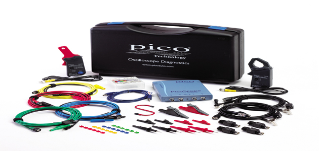
Automotive-specific scopes are now quite widely available. The main difference for these – when compared to generic types – is the packaging; often they’re in kit form and include all, or most, of the necessary interfaces and signal conditioning adaptors appropriate to automotive-type diagnostic signals.
In addition, many of them include specific features in the software to aid setting up the scope for standard automotive applications, as well as sophisticated signal analysis capability for advanced automotive diagnostics. For example, BUS system message analysis.
It is important, though, to understand the concept of how a digital scope captures the signal, as this creates a few considerations that you’ll need to think about when setting up a scope for a measurement task.
Let’s take a look at this in more detail…
Scope settings for accurate sampling
A digital sampling device – in our case a scope, but there are others in many different applications – uses something called an analogue-to-digital converter – often abbreviated to ADC – to convert the target wave form or signal to something that can be stored or manipulated by a digital signal processor or computer.
The ADC samples the applied input signal at fast, regular intervals and each sample creates a measurement value: a number that can be resolved into a binary value (1’s and 0’s) before being stored in electronic memory. In this way, we end up with a string of numbers, in memory, which represent the original waveform.
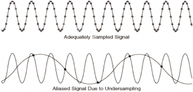
However, there is a critical consideration here: in between samples, the signal has not been measured, so, between two samples, the device simply draws a straight line known as interpolation, meaning we have to be certain that we sample enough points to capture the full signal detail.
If you don’t sample quickly enough, some detail between could be missed completely (a phenomena known as ‘aliasing’); therefore, an important consideration when setting up the scope is sampling frequency – are you sampling fast enough to capture the detail of the signal?
Of course, you could just sample every signal as fast as your device will allow, but oversampling uses up valuable memory space, and adds no value because measurement files will be unnecessarily large to manipulate and store. This part of the set-up, then, is a compromise that you’ll need to consider and get right!
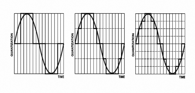
In addition, you need to think about the vertical resolution; the scope has a certain input range – for example, -10 to +10 volts. Within this range, there are a certain number of ‘bits’ – or input steps – available for the digitisation process. Effectively, this is the minimum signal change width that the scope can record between samples on the vertical axis.
This is important for a similar reason to the correct sample rate: you need to use as many available bits to digitise your signal, otherwise the digital conversion will be poor and detail will be lost.
This signal will appear ‘blocky’ with steps instead of a nice smooth curve during dynamic changes of the signal. Once you’ve got your sampling and input range setting correct, relative to the signal range you are measuring, you should then be able to enjoy measuring good quality data, which is excellent information to assist with many diagnostic procedures.
Remember to always have a good ground connection/reference on the input channel to avoid signal noise and cross-talk. Make sure also that you use the correct type of probe for the signal that you want to capture, as well as ensuring that you zero/calibrate the input channel before any real measurement. This will allow you to capture what you want, with the correct amount of detail.
Continuous learning
A further useful tip is to make sure that your scope is always on hand, primed and ready for use – not tucked away somewhere where it is an effort to be able to use it. This way it is easy to use it to measure and store signals from known good components or systems.
Furthermore, you can build up your own reference library of ‘good’ data that you can use in diagnostic procedures. Over time, this will assist you in building up a ‘big data’ set of information that can be used for comparison – particularly when you’re looking to locate a real fault. As many experienced scope users will testify, this can be an invaluable timesaver!
Of most importance, though, is the fact that you’ll need to have a good understanding of what you’re measuring, as well as knowing how to configure and use your scope effectively. Once you’ve found your feet, it is well worth getting some structured training in order to get the best out of your investment.
There are numerous providers of ‘scope’ training, but only a few that are delivered by really knowledgeable experts, who use scopes on a day-to-day basis to solve real problems.